What is a covector and what is it used for?

Addition: in a new answer I have briefly continued the explanation below to define general tensors and not just differential forms (covariant tensors).

Many of us got very confused with the notions of tensors in differential geometry not because of its algebraic structure or definition, but because of confusing old notation. The motivation for the notation $dx_i$ is perfectly justified once one is introduced to exterior differentiation of differential forms, which are just antisymmetric multilinear covectors (i.e. take a number of vectors and give a number, changing sign if we reorder its input vectors). The confusion in your case is higher because your are using $x_i$ for your basis of vectors, and $x_i$ are actually your local coordinate functions.

CONSTRUCTION & NOTATION:

Let $V$ be a finite vector space over a field $\mathbb{k}$ with basis $\vec{e}_1,...,\vec{e}_n$, let $V^*:=\operatorname{Hom}(V, \mathbb{k})$ be its dual vector space, i.e. the linear space formed by linear functionals $\tilde\omega: V\rightarrow\mathbb{k}$ which eat vectors and give scalars. Now the tensor product $\bigotimes_{i=1}^p V^*=:(V^*)^{\otimes p}$ is just the vector space of multilinear functionals $\tilde\omega^{(p)}:V^k\rightarrow\mathbb{k}$, e.g. $\tilde\omega (\vec v_1,...,\vec v_k)$ is a scalar and linear in its input vectors. By alternating those spaces, one gets the multilinear functionals mentioned before, which satisfy $\omega (\vec v_1,...,\vec v_k)=\operatorname{sgn}(\pi)\cdot \omega (\vec v_{\pi(1)},...,\vec v_{\pi(k)})$ for any permutation of the $k$ entries. The easiest example is to think in row vectors and matrices: if your vectors are columns, think of covectors as row vectors which by matrix product give you a scalar (actually its typical scalar product!), they are called one-forms; similarly any matrix multiplied by a column vector on the right and by a row vector on the left gives you a scalar. An anti-symmetric matrix would work similarly but with the alternating property, and it is called a two-form. This generalizes for inputs of any $k$ vectors.

Now interestingly, there is only a finite number of those alternating spaces: $$\mathbb{k}\cong V^0, V^*, (V^*)^{\wedge 2}:=V^*\wedge V^*,..., (V^*)^{\wedge \dim V}.$$ If you consider your $V$-basis to be $\vec{e}_1,...,\vec{e}_n$, by construction its dual space of covectors has a basis of the same dimension given by the linear forms $\tilde e^1,...,\tilde e^n$ which satisfy $\tilde e^i (\vec e_k)=\delta^i_k$, that is, they are the functionals that give $1$ only over its dual vectors and $0$ on the rest (covectors are usually indexed by superindices to use the Einstein summation convention). That is why any covector acting on a vector $\vec v=\sum_i v^i\vec e_i$ can be written $$\tilde\omega =\sum_{i=1}^n \omega_i\tilde e^i\Rightarrow \tilde\omega(\vec v) =\sum_{i=1}^n \omega_i\tilde e^i(\vec v)=\sum_{i=1}^n \omega_i\cdot v^i.$$

Finally, when you are working in differential manifolds, you endow each point $p$ with a tangent space $T_p M$ of tangent vectors and so you get a dual space $T_p^* M$ of covectors and its alternating space $\Omega_p^1(M)$ of alternating 1-forms (which in this case coincide). Analogously you define your $k$-forms on tangent vectors defining $\Omega_p^k(M)$. Since these spaces depend from point to point, you start talking about fields of tangent vectors and fields of differential $k$-forms, which vary in components (with respect to your chosen basis field) from point to point.

Now the interesting fact is that the constructive intrinsic definition of tangent vectors is based on directional derivatives at every point. Think of your manifold $M$ of dimension $n$ as given locally charted around a point $p$ by coordinates: $x^1,...,x^n$. If you have a curve $\gamma:[0,1]\subset\mathbb R\rightarrow M$ over your manifold passing through your point $p$ of interest, you can intrinsically define tangent vectors at $p$ by looking at the directional derivatives at $p$ of any smooth function $f:M\rightarrow\mathbb R$ which are given by the rate of change of $f$ over any curve passing through $p$. That is, in local coordinates your directional derivative at point $p$ along (in the tangent direction of) a curve $\gamma$ passing through it ($\gamma(t_0)=p$) is given by (using the chain rule for differentiation with the local coordinates for $\gamma (t)$): $$\frac{d f(\gamma(t))}{dt}\bigg|_{t_0}= \sum_{i=1}^n\frac{\partial f}{\partial x^i}\bigg|_p\frac{d x^i(\gamma (t))}{d t}\bigg|_{t_0}=\sum_{i=1}^n X^i\vert_p\frac{\partial f}{\partial x^i}\bigg|_p.$$ This is how that equation must be understood: at every point $p$, different curves have different "tangent vectors" $X$ with local components $X^i\vert_p\in\mathbb R$ given by the parametric differentiation of the curve's local equations (so actually you only have to care about equivalence classes of curves having the same direction at each point); the directional derivative at any point of any function in direction $X$ is thus expressible as the operator: $$X=\sum_{i=1}^n X^i\frac{\partial}{\partial x^i},$$ for all the possible components $X^i$ such that are smooth scalar fields over the manifold. In this way you have attached a tangent space $T_pM\cong\mathbb R^n$ at every point with canonical basis $\vec e_i=\frac{\partial}{\partial x^i}=:\partial_i$ for every local chart of coordinates $x^i$. This seems to be far from the visual "arrow"-like notion of vectors and tangent vectors as seen in surfaces and submanifolds of $\mathbb R^n$, but it can proved to be equivalent to the definition of the geometric tangent space by immersing your manifold in $\mathbb R^n$ (which can always be done by Whitney's embedding theorem) and restricting your "arrow"-space at every point to the "arrow"-subspace of vectors tangent to $M$ as submanifold, in the same way that you can think of the tangent planes of a surface in space. Besides this is confirmed by the transformation of components, if two charts $x$ and $y$ contain point $p$, then their coordinate vectors transform with the Jacobian of the coordinate transformation $x\mapsto y$: $$\frac{\partial}{\partial y^i}=\sum_{j=1}^n\frac{\partial x^j}{\partial y^i}\frac{\partial}{\partial x^j},$$ which gives the old-fashioned transformation rule for vectores (and tensors) as defined in theoretical physics. Now it is an easy exercise to see that, if a change of basis in $V$ from $\vec e_i$ to $\vec e'_j$ is given by the invertible matrix $\Lambda^i_{j'}$ (which is always the case), then the corresponding dual basis are related by the inverse transformation $\Lambda^{j'}_i:=(\Lambda^i_{j'})^{-1}$: $$\vec e'_j = \sum_{i=1}^n \Lambda^i_{j'}\,\vec e_i\Rightarrow \tilde e'^j = \sum_{i=1}^n (\Lambda^i_{j'})^{-1}\,\tilde e^i=:\sum_{i=1}^n \Lambda^{j'}_i\,\tilde e^i,\;\text{ where }\sum_i \Lambda^{k'}_i\Lambda^i_{j'}=\delta^{k'}_{j'}.$$ Thus, in our manifold, the cotangent space is defined to be $T_p^*M$ with coordinate basis given by the dual functionals $\omega_{x}^i (\partial/\partial x^j)=\delta^i_j$, $\omega_{y}^i (\partial/\partial y^j)=\delta^i_j$. By the transformation law of tangent vectors and the discussion above on the dual transformation, we must have that tangent covectors transform with the inverse of the previously mentioned Jacobian: $$\omega_y^i=\sum_{j=1}^n\frac{\partial y^i}{\partial x^j}\omega_x^j.$$ But this is precisely the transformation rule for differentials by the chain rule! $$dy^i=\sum_{j=1}^n\frac{\partial y^i}{\partial x^j}dx^j.$$ Therefore is conventional to use the notation $\partial/\partial x^i$ and $dx^i$ for the tangent vector and covector coordinate basis in a chart $x:M\rightarrow\mathbb R^n$.

Now, from the previous point of view $dx^i$ are regarded as the classical differentials, just with the new perspective of being the functional duals of the differential operators $\partial/\partial x^i$. To make more sense of this, one has to turn to differential forms, which are our $k$-forms on $M$. A 1-form $\omega\in T_p^*M=\Omega_p^1(M)$ is then just $$\omega = \sum_{i=1}^n \omega_i\, dx^i,$$ with $\omega_i(x)$ varying with $p$, smooth scalar fields over the manifold. It is standard to consider $\Omega^0(M)$ the space of smooth scalar fields. After defining wedge alternating products we get the $k$-form basis $dx^i\wedge dx^j\in\Omega^2(M), dx^i\wedge dx^j\wedge dx^k\in\Omega^3(M),..., dx^1\wedge\cdots\wedge dx^n\in\Omega^n(M)$, (in fact not all combinations of indices for each order are independent because of the antisymmetry, so the bases have fewer elements than the set of products). All these "cotensor" linear spaces are nicely put together into a ring with that wedge $\wedge$ alternating product, and a nice differentiation operation can be defined for such objects: the exterior derivative $\mathbf d:\Omega^k(M)\rightarrow\Omega^{k+1}(M)$ given by $$\mathbf d\omega^{(k)}:=\sum_{i_0<...<i_k}\frac{\partial\omega_{i_1,...,i_k}}{\partial x^{i_0}}dx^{i_0}\wedge dx^{i_1}\wedge\cdots\wedge dx^{i_k}.$$ This differential operation is a generalization of, and reduces to, the usual vector calculus operators $\operatorname{grad},\,\operatorname{curl},\,\operatorname{div}$ in $\mathbb R^n$. Thus, we can apply $\mathbf d$ to smooth scalar fields $f\in\Omega^0(M)$ so that $\mathbf df=\sum_i\partial_i f dx^i\in\Omega^1(M)$ (note that not all covectors $\omega^{(1)}$ come from some $\mathbf d f$, a necessary and sufficient condition for this "exactness of forms" is that $\partial_{i}\omega_j=\partial_{j}\omega_i$ for any pair of components; this is the beginning of de Rham's cohomology). In particular the coordinate functions $x^i$ of any chart satisfy $$\mathbf d x^i=\sum_{j=1}^n\frac{\partial x^i}{\partial x^j}dx^j=\sum_{j=1}^n\delta^i_jdx^j= dx^i.$$

THIS final equality establishes the correspondence between the infinitesimal differentials $dx^i$ and the exterior derivatives $\mathbf dx^i$. Since we could have written any other symbol for the basis of $\Omega_p^1(M)$, it is clear that $\mathbf dx^i$ are a basis for the dual tangent space. In practice, notation is reduced to $\mathbf d=d$ as we are working with isomorphic objects at the level of their linear algebra. All this is the reason why $\mathbf dx^i(\partial_j)=\delta^i_j$, since once proved that the $\mathbf dx^i$ form a basis of $T_p^*M$ it is straightforward without resorting to the component transformation laws. On the other hand, one could start after the definition of tangent spaces as above, with coordinate basis $\partial/\partial x^i$ and dualize to its covector basis $\tilde e^i$ such that $\tilde e^i(\partial_j)=\delta^i_j$; after that, one defines wedge products and exterior derivatives as usual from the cotangent spaces; then it is a theorem that for any tangent vector field $X$ and function $f$ on $M$ $$X(f)=\sum_{i=1}^n X^i\frac{\partial f}{\partial x^i}=\mathbf d f(X),$$ so in particular we get as a corollary that our original dual coordinate basis is in fact the exterior differential of the coordinate functions: $$(\vec e_i)^*=\tilde e^i=\mathbf d x^i\in\Omega^1(M):=T^*(M).$$ (That is true at any point for any coordinate basis from the possible charts, so it is true as covector fields over the manifold). In particular the evaluation of covectors $\mathbf d x^i$ on infinitesimal vectors $\Delta x^j\partial_j$ is $\mathbf d x^i(\Delta x^j\partial_j)=\sum_{j=1}^n\delta^i_j\Delta x^j$, so when $\Delta x^i\rightarrow 0$ we can see the infinitesimal differentials as the evaluations of infinitesimal vectors by coordinate covectors.

MEANING, USAGE & APPLICATIONS:

Covectors are the essential structure for differential forms in differential topology/geometry and most of the important developments in those fields are formulated or use them in one way or another. They are central ingredients to major topics such as:

Linear dependence of vectors, determinants and hyper-volumes, orientation, integration of forms (Stokes' theorem generalizing the fundamental theorem of calculus), singular homology and de Rham cohomology groups (Poincaré's lemma, de Rham's theorem, Euler characteristics and applications as invariants for algebraic topology), exterior covariant derivative, connection and curvature of vector and principal bundles, characteristic classes, Laplacian operators, harmonic functions & Hodge decomposition theorem, index theorems (Chern-Gauß-Bonnet, Hirzebruch-Riemann-Roch, Atiyah-Singer...) and close relation to modern topological invariants (Donaldson-Thomas, Gromow-Witten, Seiberg-Witten, Soliton equations...).

In particular, from a mathematical physics point of view, differential forms (covectors and tensors in general) are fundamental entities for the formulation of physical theories in geometric terms. For example, Maxwell's equations of electromagnetism are just two equations of differential forms in Minkowski's spacetime: $$\mathbf d F=0,\;\;\star\mathbf d\star F=J,$$ where $F$ is a $2$-form (an antysymmetric 4x4 matrix) whose components are the electric and magnetivc vector field components $E_i,\,B_j$, $J$ is a spacetime vector of charge-current densities and $\star$ is the Hodge star operator (which depends on the metric of the manifold so it requires additional structure!). In fact the first equation is just the differential-geometric formulation of the classical Gauß' law for the magnetic field and the Faraday's induction law. The other equation is the dynamic Gauß' law for the electric field and Ampère's circuit law. The continuity law of conservation of charge becomes just $\mathbf d\star J=0$. Also, by Poincaré's lemma, $F$ can always be solved as $F=\mathbf d A$ with $A$ a covector in spacetime called the electromagnetic potential (in fact, in electrical engineering and telecommunications they always solve the equations by these potentials); since exterior differentiation satisfies $\mathbf{d\circ d}=0$, the potentials are underdetermined by $A'=A+\mathbf d\phi$, which is precisely the simplest "gauge invariance" which surrounds the whole field of physics. In theoretical physics the electromagnetic force comes from a $U(1)$ principal bundle over the spacetime; generalizing this for Lie groups $SU(2)$ and $SU(3)$ one arrives at the mathematical models for the weak and strong nuclear forces (electroweak theory and chromodynamics). The Faraday $2$-form $F$ is actually the local curvature of the gauge connection for those fiber bundles, and similarly for the other forces. This is the framework of Gauge Theory working in arbitrary manifolds for your spacetime. The only other force remaining is gravity, and again general relativity can be written in the Cartan formalism as a curvature of a Lorentz spin connection over a $SO(1,3)$ gauge bundle, or equivalently as the (Riemannian) curvature of the tangent space bundle.

The answers here are all excellent and in depth, but I might also admit, a little abstract and intimidating. I'd like to present a concrete reason for covectors to exist: to make the concept of dot product invariant to coordinate transformations.

Let's say we have some point $p$ on a manifold $M$ with a vector $V$ coming off of $p$. This vector has a length, that is independent of what local coordinate system you represent it with around $p$. We might be doing computations on that length as we "transport" the vector along points on the manifold, therefore we want to base our computational machinery in operations that ignore what the local coordinates are doing and only focus on absolute quantities. To normally compute the length of a vector, you might use a dot product with itself and take the square root, but I'll show here that the dot product is vulnerable to changes in coordinate systems. That will be why I bring in covectors to solve this problem - though the difference is very subtle.

Definition of vector

Let $\mathbf p$ be the position of a point $p$. We can set up a local coordinate basis by taking the vectors that result from varying $\mathbf p$ by varying each coordinate $x_i$ while holding the others constant, i.e. taking the partial derivative $\frac{\partial \mathbf p}{\partial x_i}$. A vector at $p$ can therefore be written in terms of that basis

$$ V = \sum_i v_i \frac{\partial \mathbf p}{\partial x_i} .$$

If we switch local coordinate systems to $x_i'$ then via the chain rule we get the relationship:

$$ V = \sum_i v_i \frac{d \mathbf p}{d x_i} = \sum_i v_i \sum_j \frac{dx_j'}{dx_i} \frac{d \mathbf p}{d x_j'} = \sum_i \left ( \sum_j v_j\frac{dx_i'} {dx_j}\right) \frac{d \mathbf p}{d x_i'} =\sum_i v_i' \frac{d \mathbf p}{d x_i'} $$

which means that $$v_i' = \sum_j \frac{dx_i'}{dx_j} v_j ,$$ so we've essentially multiplied by the Jacobian matrix $J$ of the transformation. Writing $v$ and $v'$ as column vectors we get the relation

$$ v' = Jv.$$

Problem with length of vector as we change coordinate systems

Let's say we have a vector $V = 1 \hat x + 1 \hat y$. The length of this vector is $\sqrt{V \cdot V} = \sqrt{1+1} = \sqrt{2}$. Now lets scale the local coordinate system down by 2 so that the vector becomes $V' = 2 \hat x' + 2 \hat y'$. The new length is $\sqrt{V' \cdot V'} = \sqrt{4+4} = 2\sqrt{2}$. The length has changed, because we are measuring our vector in terms of local coordinates, but we do not want that. We want a way of computing the length of the vector that is invariant to re-specifications of the local coordinate system.

Introduction to covector

A covector is simply a linear function from vectors to real numbers, $\alpha : V \to \mathbb R$. For an example of a covector, we have these functions $dx_i$. As has been said in the previous answers, $dx_i$ is not a length but a function that takes vectors and picks out the $i$th coordinate component, for example in $ \mathbb R^3 $:

$$ dx_1( A\hat e_1 + B\hat e_2 + C \hat e_3) = A.$$ $$ dx_2( A\hat e_1 + B\hat e_2 + C \hat e_3) = B.$$ $$ dx_3( A\hat e_1 + B\hat e_2 + C \hat e_3) = C.$$

These functions form a basis in the space of covectors. Every linear function from vectors to the real numbers can be written as a linear combination of these functions:

$$ \alpha(v) = \sum_i a_i dx_i(v).$$

Now if we do a coordinate change to $x_i'$ we have to take contributions from all the different

$$ \alpha(v) = \sum_i a_i dx_i(v) = \sum_i \sum_j a_i \frac{dx_i}{dx_j'} dx_j'(v) = \sum_i \left ( \sum_j a_j \frac{dx_j}{dx_i'} \right ) dx_i'(v) = \sum_i a_i' dx_i'(v) .$$

We see now that

$$ a_i' = \sum_j a_j \left ( \frac{dx_j}{dx_i'} \right )$$

Now comes the important part. If we take a covector and apply it to a vector, we basically get a dot-product:

$$ \alpha(v) = \sum_i a_i v^i = av .$$

However, when we make a coordinate transform to $x_i'$ then:

$$ \alpha(v)' = a'v' = a \frac{dx}{dx'} \frac{dx'}{dx} v = av.$$

The answer stays the same. Thus, we've found a way to compute a "dot product" that is invariant to local coordinate transformations.

Revisiting problem

When we scale the coordinate system for $V$ as in the previous problem, now we treat this as a covector being applied to a vector. Therefore upon the transform, the covector components actually half, so that the answer stays the same:

$$ |V| = \sqrt{\alpha(V)} = \sqrt{1/2*2 + 1/2 *2} = \sqrt{2} $$.

tldr covectors implement a "fix" to the dot product in differential geometry so that the result is invariant to changes of the local coordinate system.

It's always been easier for me to think of "covectors" (dual vectors, cotangent vectors, etc.) as different basis of vectors (potentially for a different space than "usual" vectors) because the linear algebra properties are still basically the same. Yeah, a covector is an object that "takes" a vector and returns a number, but you could define a vector as an object that "takes" a covector and returns a number! (And saying that this is all vectors and covectors can do--return numbers through the inner product--seems quite an understatement of what they can be used for.)

Furthermore, in a space with a metric, covectors can be constructed easily by using the tangent basis vectors.

Let $e_1, e_2, e_3$ be a tangent-space basis for a 3d real vector space. The basis covectors are then

$$\begin{align*} e^1 &= \frac{e_2 \wedge e_3}{e_1 \wedge e_2 \wedge e_3} \\ e^2 &= \frac{e_3 \wedge e_1}{e_1 \wedge e_2 \wedge e_3} \\ e^3 &= \frac{e_1 \wedge e_2}{e_1 \wedge e_2 \wedge e_3} \end{align*}$$

(These wedges simply form higher dimensional objects than vectors but that are built from vectors. $e_2 \wedge e_3$ is, for example, an oriented, planar object corresponding to the parallelogram spanned by $e_2, e_3$. Thus it is related to the cross product in 3d, but the wedge product is useful in other dimensions, too, while the cross product does not generalize outside of 3 and 7 dimensions.)

Basically, the basis covectors are formed by finding the vectors orthogonal to hypersurfaces spanned by all other basis vectors.

Covectors are useful in large part because they enter expressions through the vector derivative $\nabla$. We generally define $\nabla = e^i \partial_i$ over all $i$ to span the space.

The notation that the basis covectors are $dx_1, dx_2,\ldots$ is one I too find a bit confusing; in geometric calculus, they would either signify scalars or vectors! But I think I understand that to mean that $\nabla x^1$ extracts the $e^1$ basis covector from the vector derivative, and they are just using $d$ to mean something that might otherwise be denoted $\nabla$ (which is not uncommon, as has been pointed out, in differential forms).

$$\nabla x^1 = e^1 \frac{\partial}{\partial x^1} x^1 = e^1$$

if that makes it more clear.

Covectors are weighted averages.

Keep the same data $\vec{x}$, the same style of inner product, $$\alpha_1 \cdot x_1 + \alpha_2 \cdot x_2 + \alpha_3 \cdot x_3 \ldots$$ but change the $\alpha_i$ in the above expression. This is "adjusting weights" in everyday parlance or "moving the covector" in mathematical words. People really do do this all the time, so it's not esoteric or merely-academic. (Notice that after I sum the product-pairs I'll have one scalar answer. I've "reduced" dimension to 1 in a "map-reduce" sense. This is the way inner products work.)

You can also use the visual of a loss function to centre yourself in "parameter space". Think about you have a model with a given form $$\alpha_1 \cdot \phi_1(\vec{x}) + \alpha_2 \cdot \phi_2(\vec{x}) + \alpha_3 \cdot \phi_3(\vec{x}) + \ldots$$ for example the $\phi_i$ could be basis functions. Adjusting the weights $\alpha_i$ is the goal of statistical modelling. For example the OLS solution picks an "optimal" covector (in some sense of the word "optimal"). And gradient descent on some kind of model that can be parameterised by "summed weightings of [stuff]" is also shooting for the same goal by exploring the covector space.

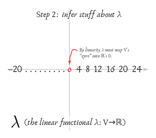
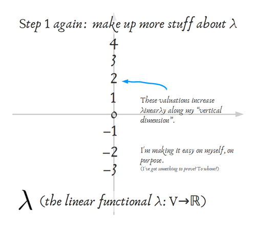
Regarding your question about $dx_i$ (projection functions on the $i$th dimension: forgetting every other coordinate but the $i$th). Go back to the top equation I wrote $\sum \alpha_i \cdot x_i$. Set all of the $\alpha_i$'s to zero except for $\alpha_1$. Now as you increment $\alpha_1$ what happens algebraically? You get $$\{\alpha_1=1\} \implies \sum=x_1; \quad \{ \alpha_1=2\} \implies \sum=2x_1; \quad \cdots $$ (What is that geometrically? It's slopes increasing the same way as in calc 101. Except we'll be able to combine that with the outcomes of the other $\alpha_{j\neq 1}$ in a second) If you set any of the $\alpha_{j \neq i}$ to zero and raised one "slider" $\alpha_i$ at a time you'd find the same thing. And because of linear-algebra I know I can, except in a few bad cases, "straighten" the basis so it's orthonormal (unshear, rotate, whatever...Gram-Schmidt fixes it automatically), meaning the $\alpha_i$'s will operate independently (linearly-independently--sum-of-products style) of each other and you can actually infer every number in the induced scalar-field all over the space, from the axes (even from just the first step out on any given axis).

I found it helpful to draw a plane and work it out by hand (I agree with you, @Mike, that $\mathbb{R}^2$ is the way to start) with a really simple example.

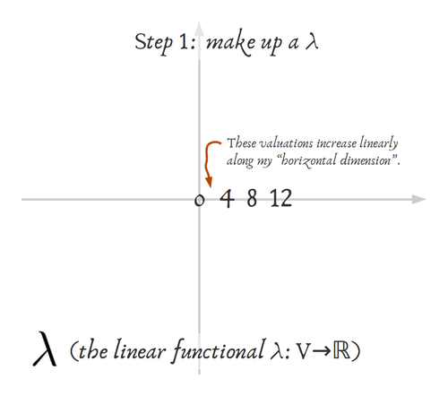
In the example I drew, I chose $\alpha_1=4$ and $\alpha_2=1$ but the point is that, however you do this,

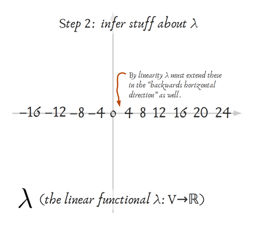
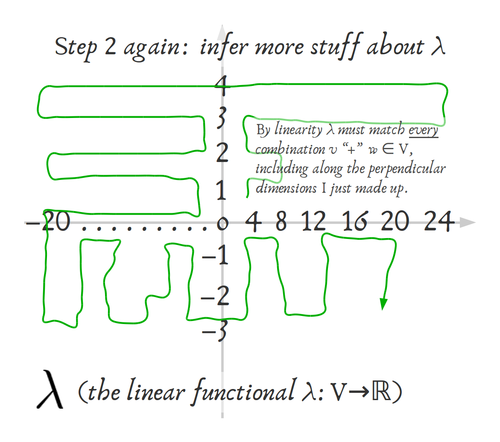
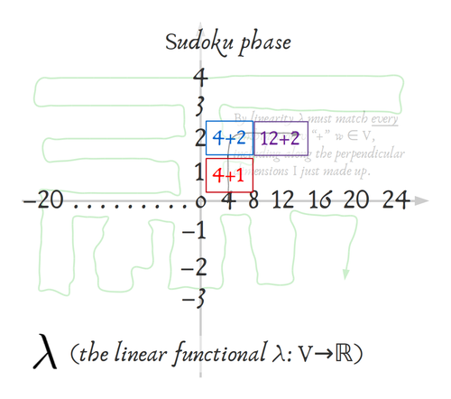
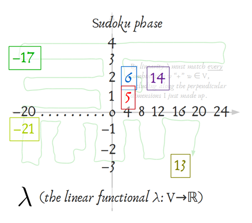
Eventually as I unwind the definition more-and-more, with really simple numbers on something drawable, I found the familiar "level sets" -- so the linear structure is showing up again in the scalar-field (dual space). Yay!

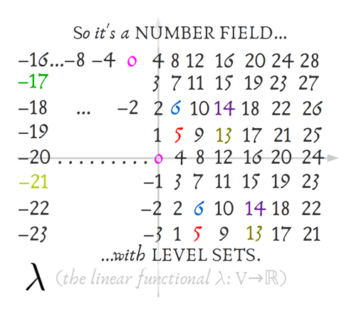
And as you think about the ways this scalar-field could change (what would have happened if you changed some of the $\alpha_1 \text{ or } \alpha_2$), you might start to see why Wikipedia used the stack-of-hyperplanes visual for their entry....

HTH

There are at least two layers of ideas here. First, as you say, the "dual space" $V^*$ to a real vector space is (by definition) the collection of linear maps/functionals $V\rightarrow \mathbb R$, with or without picking a basis. Nowadays, $V^*$ would more often be called simply the "dual space", rather than "covectors".

Next, the notion of "tangent space" to a smooth manifold, such as $\mathbb R^n$ itself, at a point, is (intuitively) the vector space of directional derivative operators (of smooth functions) at that point. So, on $\mathbb R^n$, at $0$ (or at any point, actually), $\{\partial/\partial x_1, \ldots, \partial/\partial x_n\}$ forms a basis for that vector space of directional-derivative operators.

One notation (a wacky historical artifact, as you observe!) for the dual space to the tangent space, in this example, is $dx_1,\ldots, dx_n$. That is, literally, $dx_i(\partial/\partial x_j)$ is $1$ for $i=j$ and $0$ otherwise.

One way to help avoid some confusions is to not be hasty to identify all $n$-dimensional real vector spaces with $\mathbb R^n$, so that you don't feel an obligation to evaluation $dx_1(a,b)$... even though, if you view $(a,b)$ as $a\cdot \partial/\partial x_1 + b\cdot \partial/\partial x_2$, then $dx_1$ evaluated on it gives $a$.

As much as anything, this is just a notational set-up for calculus-on-manifolds that includes various historical artifacts that are somewhat incompatible with other notational conventions, I agree! For example, just when you get used to the idea that in $dy/dx$ the $dy$ and the $dx$ cannot be separated, that seems to have been done in writing a differential form $f(x,y)dx+g(x,y)dy$. And, in fact, the latter notation descends from a tradition that was not fussing about whether there were or weren't infinitesimals and all that, and would perform such symbolic manipulations, for one thing. That is, in my opinion, even on $\mathbb R^n$, the notation is best understood, for what it is meant to suggest, not in a contemporary context, but imagining ourselves in 1890 or so. This is a separate issue from those about proving things, of course, but may be helpful in intepreting the intention of the notation.